
With LLMs around, I feel like I haven't been writing as much code as I used to. I figured a good way to keep the coding part of my brain active, and to make sure I don't forget how to do math, was to get back into reading papers and implementing them. So I wanted to start a series of blog posts on the papers I find interesting. The paper I'm digging into for this post, Generating interpretable rainfall-runoff models automatically from data, is a great one to start the series with. It's one of my favorite papers from the last few years. It's from a grad school friend of mine, Travis Dantzer. If you enjoy good math and water, go check out the rest of his work, it's phenomenal.
These blog posts will be broken into three sections:
What is the paper about, what problem is it addressing, and what makes this work novel.
What are the core ideas introduced in the paper, and the methodology implementation in Python.
Where do we go from here. This will go over related papers and my hot takes.
Problem statement
One of the fundamental problems in urban water and hydrology is predicting runoff from a catchment during a rain event. What we call a “catchment” changes a bit in an urban setting, but the goal remains the same: predict the flow at a location based on previous flow measurements and rainfall data. This problem has been studied since forever. At the fundamental level, all these methods attempt to find the function that maps precipitation to runoff.
The advancements over the years have been about defining the nature of that function. In the 1930s, people came up with the unit hydrograph approach for predicting catchment runoff response. This approach is still the workhorse for these problems in both the natural and built environment. More recently, research has moved toward neural network-based approaches. You can think of the state-of-the-art in runoff prediction as a spectrum from “physics” based approaches on one end to pure data-driven approaches on the other. There’s no free lunch: the rigidity of the linear assumption in the unit hydrograph limits accuracy, and neural networks trade interpretability for it. It’s a knob where you get one or the other. Most researchers have been leaning toward the ML side and then trying to bolt interpretability back on by explaining weights and model behavior after the fact.
This is where this paper comes in, Generating interpretable rainfall-runoff models automatically from data introduces a new methodology, MOdel Discovery in Partially Observable Dynamical Systems (modpods), that is kind of a Goldilocks approach between ML and classical physical models. This approach is interpretable and has good accuracy, not far off the best neural networks. The novelty of the methodology lies in how it accounts for the lag between rainfall and runoff response, and in its use of a SINDy-inspired approach for learning the equations representing the system dynamics. More on this in the next section.
Core Ideas
The core ideas in the paper can be summarized as follows:
Using a gamma distribution function to account for the rainfall response lag and transform rainfall into the catchment’s hidden states.
Using a polynomial to approximate the gradient (the time derivative) of the runoff.
Formulating a nested optimization problem: a SINDy-inspired least squares approach to identify the polynomial coefficients, and an outer optimization loop that finds the gamma parameters (and how many of them you need).
Rainfall-runoff lag
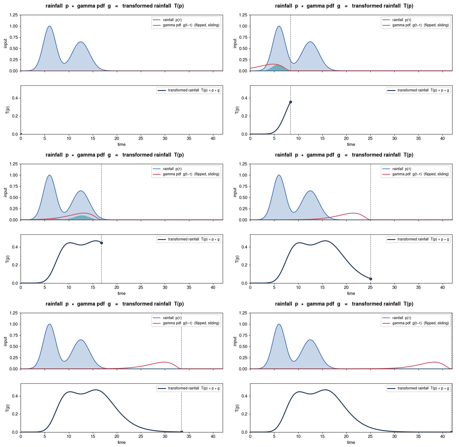
One of the main challenges in learning a rainfall-runoff mapping is representing the lag between rainfall and its runoff response. If you train a neural network to predict runoff, you have to engineer how much rainfall the model gets to see: the last 12 hours, 24 hours, etc. It's not an intractable problem, but it's one more thing you have to get right. modpods introduces an elegant convolution-based approach for representing this lag. This approach uses a gamma probability density function (PDF) to transform rainfall intensity into a latent variable that we'll use for learning the runoff response. The gamma PDF, represented by the equation below, has three parameters, and each one means something physical: alpha is the shape/skew, beta is the rate (decreasing beta delays and broadens the peak), and d is a pure time delay. (The timing of the peak actually depends on all three together, but d is the clean time shift.) The shape of the gamma PDF is the red line in the animation below.
When we have a rainfall event, we take its convolution with the gamma PDF. The idea is that the transformed signal at any point depends on all of the rainfall that came before it. In practice, the tail zeros out numerically after a while, but in theory the gamma's tail runs off to infinity. The animation below illustrates this idea better. The top row represents the rainfall (in blue) and the gamma PDF (in red), and the second row represents the convolved output. You can think of the convolved signal at time t as the area of interaction between the rainfall before t and the gamma curve. This effectively transforms rainfall into a latent variable that is a "gamma-weighted sum" of the rainfall. modpods formulates this gamma function as something we can learn from data.
In modpods, instead of one unit hydrograph representing the whole catchment, like most classical approaches do, we say the catchment is characterized by several. Each one is an "effective subcatchment," and we learn a gamma PDF for each of these subcatchments. We then combine these responses to estimate the net hydrograph. This idea is very similar to the RTK approach. You can also think about it like a Fourier decomposition: there you convert a signal into fixed sine and cosine basis functions; here we transform the rainfall by gamma convolution into a new basis and then learn the dynamics in that basis (though unlike Fourier, this basis is learned, not fixed). That analogy helped me better understand this approach.
Learning the dynamics using a polynomial
Now that we have a gamma transformed basis Ti(po), where Ti is the gamma transformation and po is the precipitation, modpods writes the dynamics equation as a polynomial in qo, po, and a polynomial of the transformed p. You usually need that autoregressive component (the terms in qo) to anchor the dynamics; it’s what captures the recession curve. The general form is listed shown below equation.
The most complex version trained in the paper (third order polynomial, two effective subcatchments) looks like:
The one constraint worth knowing is that the highest order autocorrelation term has to be negative, so that finite rainfall produces a finite, decaying response instead of blowing up. In my tests, imposing this constraint made a drastic difference to the stability of the method.
One of the interesting things to note about this formulation is that unlike classical methods, where we directly map runoff to rainfall, modpods uses a SINDy-inspired formulation where the gradient of the system is represented as a linear combination of nonlinear basis functions. If you want to learn more about SINDy, check out my previous post.
Nested optimization loop to estimate parameters
For a given catchment's rainfall-runoff dataset, modpods is parametrized by polynomial coefficients and gamma PDF parameters. The total number of parameters is:
where m is the number of subcatchments and q is the polynomial order. That works out to 6 parameters for the simplest model and 18 for the most complex one in the paper (m=2, q=3).
These parameters are estimated using a nested optimization loop. The inner loop uses a least squares variant (the SINDy step) to find the polynomial coefficients that best fit the differential equation described above. The outer loop then iterates over combinations of parameters: the number of subcatchments and the parameters defining each gamma function. This loop repeats until the fit stops improving; in the paper, it keeps adding subcatchments until the next one improves the fit by less than 0.5%. The paper uses compass search for this. I’ve been using Bayesian optimization through Optuna instead, mostly because it was a little easier to wire up and it’s more sample-efficient over the messy, non-convex space of gamma parameters.
Official implementation of the MODPODS is available at https://github.com/dantzert/modpods/tree/main. The implementation in this post is a simple example I wrote to help me better understand the methodology.
Cool plots!!
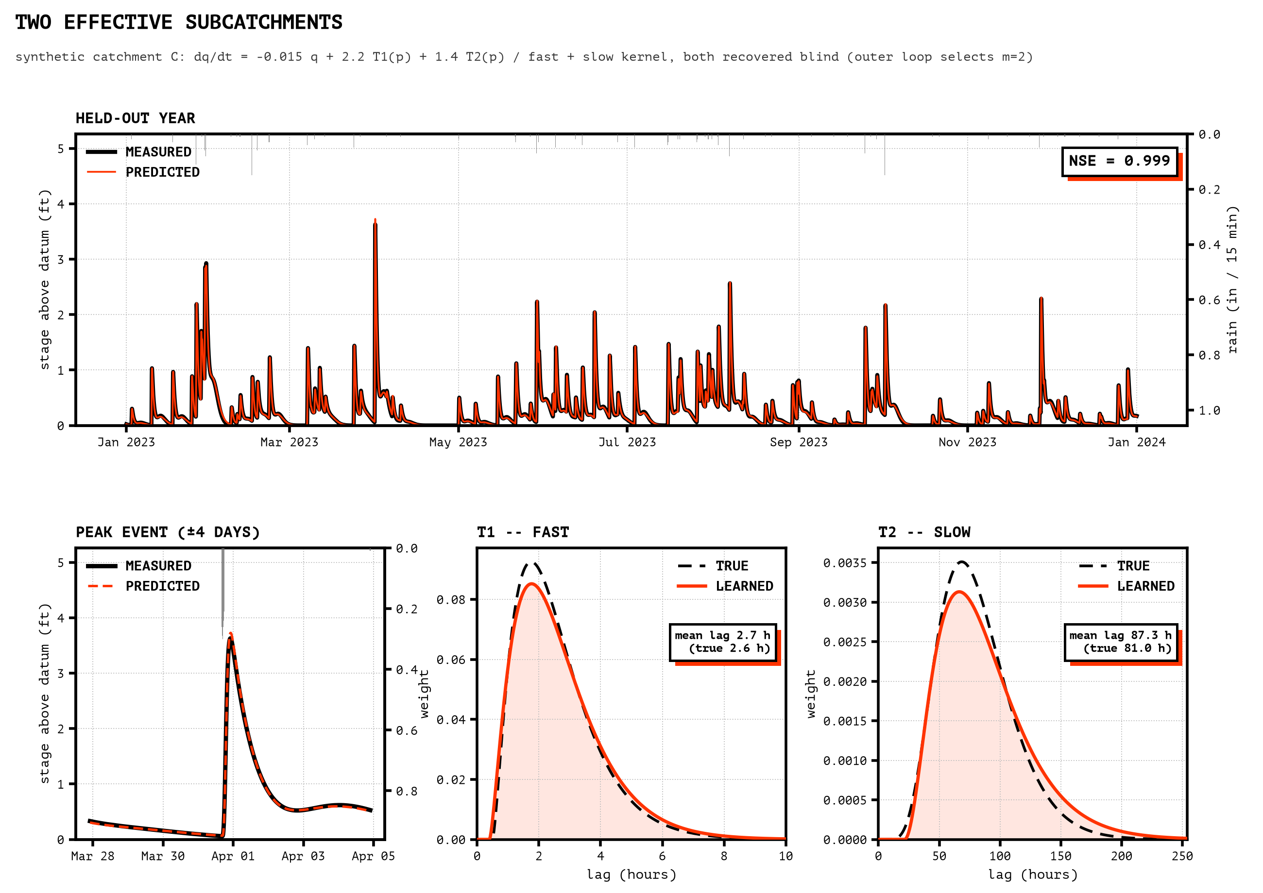
This is a synthetic example where I fit a synthetic hydrograph generated using a combination of a fast (~8 hours) and a slow (~200 hours) kernel. modpods is able to latch on to this almost perfectly. I used a simple test case like this to make sure my implementation is correct. It is amazing how good the fit is for fewer than 10 model parameters.
Where do we go from here?
Thanks for reading so far! It has been a long post. But if you stuck around till here, please do read this paper, and also check out the SINDy paper.
The main thing I keep coming back to is that this should extend pretty cleanly to urban water systems. I’ve been using a Gaussian process to learn the diurnal (dry weather) response and then modpods to learn the wet weather response on top of it. If that combination sounds interesting, check out An automated toolchain for the data-driven and dynamical modeling of combined sewer systems by another lab mate of ours, Sara Troutman.
The other direction I want to try is changing how we represent the gradient. Right now it’s a polynomial, but other function families may do a better job on the residuals, especially on the recession limb where a polynomial can struggle.
Disclaimer: LLMs were extensively used to fix grammatical and typographical errors, develop the code snippet, and style the plot.
Python Implementation
import numpy as np
import pandas as pd
import matplotlib.pyplot as plt
import optuna
from scipy.integrate import solve_ivp
from scipy.signal import fftconvolve
from scipy.stats import gamma


def gamma_pdf(x, alpha, beta, d=0.0):
    # beta is a rate (paper eq. 1), so scipy scale = 1/beta
    return gamma.pdf(x, a=alpha, scale=1/beta, loc=d)


def transform_rain(rain, alpha, beta, d=0.0):
    kernel = gamma_pdf(np.arange(len(rain)), alpha, beta, d)
    return fftconvolve(rain, kernel)[:len(rain)]


def build_feature_matrix(stage, rain, transforms, poly_order=3):
    base = np.column_stack([stage, rain, *transforms])
    base_names = ['q', 'p'] + [f'T{i+1}(p)' for i in range(len(transforms))]
    theta = np.hstack([base**k for k in range(1, poly_order + 1)])
    names = [n if k == 1 else f'{n}^{k}' for k in range(1, poly_order + 1) for n in base_names]
    return theta, names


def fit_and_score(stage, rain, gamma_params, poly_order, windup, bibo_stable=False):
    transforms = [transform_rain(rain, a, b, d) for a, b, d in gamma_params]
    theta, names = build_feature_matrix(stage, rain, transforms, poly_order)
    dq = np.gradient(stage, edge_order=2)
    theta, dq = theta[windup:], dq[windup:]
    if not np.all(np.isfinite(theta)):
        return None, None, -1.0
    if bibo_stable:
        # coefficient on the highest power of q must be <= 0 (paper sec 4.1)
        from scipy.optimize import lsq_linear
        upper = np.full(theta.shape[1], np.inf)
        upper[(poly_order - 1) * (2 + len(gamma_params))] = 0.0
        xi = lsq_linear(theta, dq, bounds=(-np.inf, upper)).x
    else:
        xi, *_ = np.linalg.lstsq(theta, dq, rcond=None)
    residual = dq - theta @ xi
    r2 = 1 - np.sum(residual**2) / np.sum((dq - dq.mean())**2)
    return xi, names, r2


def suggest_gamma_params(trial, num_transforms):
    params = []
    for i in range(num_transforms):
        alpha = trial.suggest_float(f"alpha_{i+1}", 1.0, 50.0, log=True)
        beta = trial.suggest_float(f"beta_{i+1}", 1/1000, 2.0, log=True)
        d = trial.suggest_float(f"d_{i+1}", 0.0, 96.0)
        params.append([alpha, beta, d])
    return np.array(params)


def train(stage, rain, windup, poly_order=3, max_transforms=2, n_trials=1500, min_gain=0.005, seed=0):
    optuna.logging.set_verbosity(optuna.logging.WARNING)
    results = {}
    for m in range(1, max_transforms + 1):
        print(f"training with {m} transformation(s)")

        def objective(trial):
            gamma_params = suggest_gamma_params(trial, m)
            return fit_and_score(stage, rain, gamma_params, poly_order, windup)[2]

        study = optuna.create_study(direction="maximize",
                                    sampler=optuna.samplers.TPESampler(seed=seed + m))
        study.enqueue_trial({f"{k}_{i+1}": v for i in range(m)
                             for k, v in zip(("alpha", "beta", "d"), (1.0, 1.0, 0.0))})
        if m > 1:
            # seed the new kernel at several timescales, TPE won't find slow ones alone
            warm = dict(results[m - 1]['study'].best_params)
            for beta_new in (0.3, 0.05, 0.02, 0.01, 0.005):
                study.enqueue_trial(warm | {f"alpha_{m}": 3.0, f"beta_{m}": beta_new, f"d_{m}": 0.0})
        study.optimize(objective, n_trials=n_trials)

        gamma_params = np.array([[study.best_params[f"alpha_{i+1}"],
                                  study.best_params[f"beta_{i+1}"],
                                  study.best_params[f"d_{i+1}"]] for i in range(m)])
        xi, names, r2 = fit_and_score(stage, rain, gamma_params, poly_order, windup)
        results[m] = {'gamma_params': gamma_params, 'xi': xi, 'feature_names': names,
                      'r2': r2, 'study': study}
        print(f"  m={m}: R^2 = {r2:.5f}")
        if m > 1 and r2 < results[m - 1]['r2'] + min_gain:
            print(f"  marginal gain < {min_gain}, keeping m={m-1}")
            break
    return results


def simulate(stage, rain, transforms, xi, poly_order, windup):
    # integrate dq/dt with scipy, forcing held constant across each timestep
    forcing = np.column_stack([rain, *transforms])[windup:]
    obs = stage[windup:]
    n = len(obs)

    def f(t, q):
        base = np.concatenate((q, forcing[min(int(t), n - 1)]))
        return [np.concatenate([base**k for k in range(1, poly_order + 1)]) @ xi]

    # max_step=1: the forcing is piecewise constant, adaptive steps must not skip a timestep
    sol = solve_ivp(f, (0, n - 1), [obs[0]], t_eval=np.arange(n), max_step=1.0)
    q = np.full(n, np.nan)
    q[:len(sol.t)] = sol.y[0]
    return q


def nash_sutcliffe(obs, sim):
    ok = np.isfinite(obs) & np.isfinite(sim)
    return float(1 - np.sum((obs[ok] - sim[ok])**2) / np.sum((obs[ok] - obs[ok].mean())**2))


# synth_c_two_kernels: dq/dt = -0.015 q + 2.2 T1(p) + 1.4 T2(p), truth in data/synth_truth.json.
# already causally aligned (no rain shift) and zero-referenced
data = pd.read_csv("./data/synth_c_two_kernels.csv", index_col='datetime', parse_dates=True)[['rain_in', 'stage']]

# train on 2022, hold out 2023, 30 days of convolution windup on each segment
test_start = pd.Timestamp("2023-01-01", tz="UTC")
train_data = data.loc[:test_start].iloc[:-1]
windup = train_data.index.get_loc(train_data.index[0] + pd.Timedelta(days=30))
test_data = data.loc[test_start - pd.Timedelta(days=30):]
test_windup = test_data.index.get_loc(test_start)

if __name__ == "__main__":
    results = train(train_data.stage.values, train_data.rain_in.values, windup)
    res = results[max(results)]

    print("\nidentified model:")
    for i, (a, b, d) in enumerate(res['gamma_params']):
        print(f"  T{i+1}: alpha={a:.3f}, beta={b:.5f}, d={d:.1f}  (mean lag {a/b + d:.0f} timesteps)")
    for name, coef in zip(res['feature_names'], res['xi']):
        print(f"  {name:10s} {coef:+.6f}")

    transforms = [transform_rain(test_data.rain_in.values, a, b, d)
                  for a, b, d in res['gamma_params']]
    sim = simulate(test_data.stage.values, test_data.rain_in.values, transforms,
                   res['xi'], 3, test_windup)
    obs = test_data.stage.values[test_windup:]
    nse = nash_sutcliffe(obs, sim)
    print(f"\nheld-out year NSE = {nse:.3f}")

    fig, ax = plt.subplots(figsize=(12, 4))
    t = test_data.index[test_windup:]
    ax.plot(t, obs, color='#1b1b1b', lw=1.0, label='measured')
    ax.plot(t, sim, color='#ff3300', lw=1.0, label='predicted')
    ax.set_ylabel("stage above datum (ft)")
    ax.set_title(f"held-out year -- NSE = {nse:.3f}")
    ax.legend()
    fig.tight_layout()
    fig.savefig("figures/predicted_vs_measured.png", dpi=150)
    print("wrote figures/predicted_vs_measured.png")
As always, I learned something new & interesting. Keep writing!
you know lots of things, its cool.