discovering governing equations from data

numpy implementation of SINDy by Brunton et.al.

Rothko says that his images are meant to represent basic emotions that encapsulate the human experience. However, Rothko’s work always reminds me of sparse matrices. I thought a Rothko might be the best way to capture what I am trying to convey in this post 😆. Rothko (No. 3/No. 13)

Lately, I have been wanting to go back to classical data-driven methodologies to review these methods and flex the math part of my brain that has atrophied from doing a bit too much programming and very little math 😅. So I wanted to write a series of blog posts about math I find fascinating.

I’m a huge fan of Dr. Burton YouTube channel. His lectures on data-driven analysis are amazing! His book, Data Driven Science and Engineering, is one of my personal favorites. In this post, I want to discuss one of his works, Discovering governing equations from data: Sparse identification of nonlinear dynamical systems. This paper introduces a methodology for discovering the underlying dynamical system based on observations. Their group also developed a Python library, pySINDy, that implements this methodology. I have reimplemented it from scratch in this post to just help better understand the algorithm.

Sparse Identification of Nonlinear Dynamical Systems (SINDy)

The main crux of this approach is the understanding that governing equations in most physical systems are sparse in non-linear high-dimensional spaces. Similar to the Kernel Trick, we project observations into a non-linear function space (e.g., sin(x), polynomial(x)) to create a set of basis vectors, and then identify the combination that approximates the underlying system of equations. This might make more sense as we dig into the methodology.

methodology

Consider the general form of a dynamical system, where f(x) represents the underlying dynamical system.

\(\frac{d}{dt} x = \mathbf{f}(x)\)

In SINDy, we approximate the dynamical system as a linear combination of non-linear basis functions.

\(\mathbf{f}(x) = \sum^p_{k=1} \theta_k(x) \xi_k = \Theta \xi \)

theta is the matrix of basis functions, and epsilon is the corresponding coefficients.

\(\Theta( \mathbf{X}) = \begin{bmatrix} 1 & \mathbf{X} & \mathbf{X}^2 & sin(\mathbf{x}) & cos(\mathbf{x}) & \dots \end{bmatrix}\)

Basis functions can be anything. They can be sin(x), x2, exponential function, etc.

\(\dot{\mathbf{X}} = \Theta(\mathbf{X}) \xi\)

We then compute the numerical gradient of observations; this can be done through good old finite differences, and then estimate the coefficients by solving the following equation.

\(\xi = \underset{\xi}{\mathrm{argmin}} || \dot{\mathbf{X}} - \Theta \xi||_2 + \lambda || \xi ||_1\)

implementation

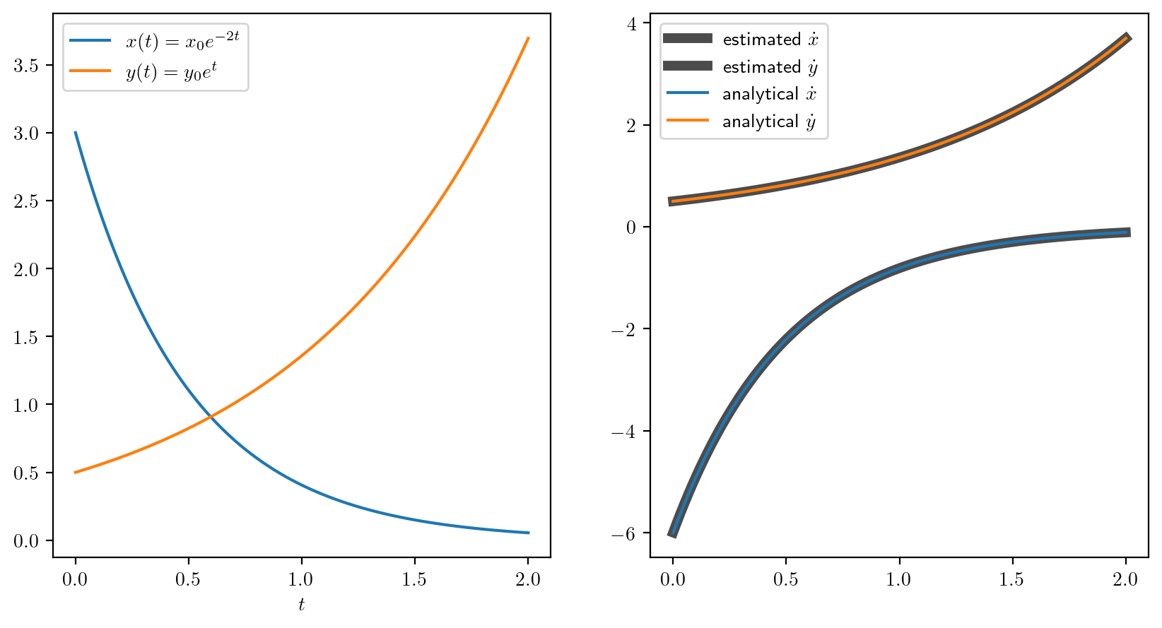
SINDy might make more sense once you look at the code. In this example, we will see how we can use this approach to determine the dynamical system by just observing the data generated by the following equations.

\(x(t) = x_0 e^{-2t}; y(t) = y_0 e^{t}\)

The analytical gradient of these equations is very straightforward (see the equations below). We will validate the dynamical system identified by SINDy with these analytical equations.

\(\dot{x}(t) = -2 x_0 e^{-2t}; \dot{y}(t) = y_0 e^t\)

Lets take a look at the code,

import numpy as np
import matplotlib.pyplot as plt
plt.rcParams['text.usetex'] = True


def numerical_gradient(x: np.ndarray, t: np.ndarray) -> np.ndarray:
    """
    estimate numerical gradient of x with respect to t
    using central difference for interior points and forward/backward    for endpoints.
    """
    df = np.zeros(len(t))
    df[0] = (x[1] - x[0]) / (t[1] - t[0])
    df[-1] = (x[-1] - x[-2]) / (t[-1] - t[-2])
    for i in range(1, len(t)-1):
        df[i] = (x[i + 1] - x[i - 1]) / (t[i + 1] - t[i - 1])
    return df

# generate synthetic data
t = np.linspace(0, 2, 120)
x0 = 3
y0 = 0.5
x = x0 * np.exp(-2.0 * t)
y = y0 * np.exp(t)

# estimate the numerical gradient
dxdt = numerical_gradient(x, t)
dydt = numerical_gradient(y, t)

# generate the basis functions for the SINDy algorithm, we will use polynomial basis functions
basis = np.vstack([np.ones_like(x), x, y, x*y, (x**2) * y, x * (y**2), x**2, y**2, x**3, y**3]).T

# solve the least squares problem to find the coefficients
# get the initial guess for the coefficients
dX = np.vstack([dxdt, dydt]).T
epsi = np.linalg.lstsq(basis, dX, rcond=None)[0]
# this the cutoff value for the coefficients
lmda = 0.7
iterations = 10
dimensions = 2
for i in range(iterations):
    indx = np.abs(epsi) < lmda
    epsi[indx] = 0.0
    for dim in range(dimensions):
        basis_index = indx[:, dim] == False
        epsi[basis_index, dim] = np.linalg.lstsq(basis[:, basis_index], dX[:, dim], rcond=None)[0]

print("Estimated coefficients: \n", epsi)

# analytical solution for the differential equations
x_dot_analytical = -2 * x0 * np.exp(-2 * t)
y_dot_analytical = y0 * np.exp(t)

# plot the results
plt.figure(1, figsize=(10, 5), dpi=200)
plt.subplot(1, 2, 1)
plt.plot(t, x, label='$x(t) = x_0 e^{-2t}$')
plt.plot(t, y, label='$y(t) = y_0 e^{t}$')
plt.xlabel(r'$t$')
plt.legend()

plt.subplot(1, 2, 2)
x_estimated = np.dot(basis, epsi[:, 0])
y_estimated = np.dot(basis, epsi[:, 1])
plt.plot(t, x_estimated, label=r'estimated $\dot{x}$', lw=5, alpha=0.7, color='k')
plt.plot(t, y_estimated, label=r'estimated $\dot{y}$', lw=5, alpha=0.7, color='k')
plt.plot(t, x_dot_analytical, label=r'analytical $\dot{x}$')
plt.plot(t, y_dot_analytical, label=r'analytical $\dot{y}$')
plt.legend()
plt.savefig("pysindy_example.png", bbox_inches='tight')

We can see that SINDy is able to approximate the coefficients pretty well. These coefficients mean that x and y, the second and third columns, in the basis matrix are enough to approximate the underlying differential equation.

Estimated coefficients: 
 [[ 0.          0.        ]
 [-1.99819104  0.        ]
 [ 0.          0.99976947]
 [ 0.          0.        ]
 [ 0.          0.        ]
 [ 0.          0.        ]
 [ 0.          0.        ]
 [ 0.          0.        ]
 [ 0.          0.        ]
 [ 0.          0.        ]]

The above can be interpreted as,

\(\dot{x} = -1.998x ; \dot{y} = 0.999 y\)

In the following plot, we can see that the estimate of the gradient is pretty close to the analytical gradient.

final thoughts

I really like the elegance of this approach. This idea is very similar to the kernel trick that is used in Gaussian Process for generalizing them. Though there might be some skill involved in choosing the right set of basis functions, it is not too hard if we have a sense of dynamics in the physical system.

I think this approach would be great for calibration of process engineering models in wastewater systems. I think SINDy provides a clean way to integrate ASM models’ equations as basis vectors.

I hope you found this post useful.

Thanks for reading 🫶🏽

---

🎧 - I am currently obsessed with Digitalism.

📖 - I am reading The Man in the High Castle.